Introduction to R and RStudio

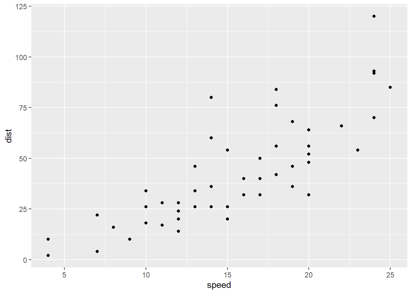
R is a free, open-source language for data manipulation, analysis, and visualization. RStudio is the IDE (workbench) that makes R friendlier and faster. Together they give you a modern workflow for reproducible research in mass communication.

Use R for the statistics and graphics; use RStudio to write code, render reports, manage files, and keep projects organized.

What is R?

A programming language for statistics and data work (from simple summaries to machine learning).
Script-based: you write code that documents exactly what you did—great for transparency and reuse.
Superpowers via packages (e.g., tidyverse for wrangling, ggplot2 for visualization).

Why it matters here: You’ll analyze surveys, scrape or analyze social media, and make publication-quality figures—repeatably.

What is RStudio?

RStudio (by Posit) is the integrated development environment for R:

Source editor with syntax highlighting and autocomplete
Console for running code
Environment to inspect objects/datasets
Files/Plots/Packages/Help/Viewer to manage outputs and docs
Tight integration with Quarto (dynamic documents) and Git

Outcome: faster iteration, cleaner organization, and easier collaboration.

Why Use R + RStudio?

Open Source

Free to install and extend. A huge community keeps adding new methods without license fees.

Analysis & Visualization

From descriptive stats to regression and beyond in one place; ggplot2 produces clear, customizable graphics.

Reproducible Research

Quarto documents combine text + code + output in one file. Re-render to update everything automatically.

Flexible & Extensible

Thousands of packages for text analysis, social media data, networks, etc. Write your own functions when needed.

Install R and RStudio

1) Install R

Go to https://cran.r-project.org/
Choose your OS (Windows / macOS / Linux) and install.

2) Install RStudio

Go to https://posit.co/download/rstudio-desktop/
Download RStudio Desktop (free) for your OS and install.

Install R first, then RStudio. RStudio detects your R installation at launch.

Meet the RStudio Interface (Four Panes)

Source (top-left): write/edit scripts (.R) and Quarto files (.qmd).
Console (bottom-left): run code interactively; see results/errors.
Environment (top-right): objects in memory (data frames, models, etc.).
Output (bottom-right): Files, Plots, Packages, Help, Viewer (for HTML/Shiny/Quarto previews).

For a deeper tour, see RStudio’s Four Panes in this section.

Start a New Project

Projects keep everything for one assignment/research task in one folder.

File → New Project…
Choose New Directory → New Project (or link an existing folder).
Name it and create.

Benefits: consistent working directory, clean file paths, and fewer “where did that file go?” moments. Git can be enabled during setup for version control.

File Management Essentials

R Script vs. R Markdown / Quarto

R Script (.R): pure code; great for fast analysis.
Quarto (.qmd): prose + code + output → renders to HTML/PDF/Word for reports.

# R Script example
summary(cars)
plot(cars)

# Quarto example chunk (runs when you render the doc)
library(ggplot2)
ggplot(cars, aes(speed, dist)) + geom_point()

CSV vs. Excel

Prefer CSV for clean, durable data.
Use Excel only when collaborators require it or you genuinely need multiple sheets.

Suggested subfolders

data/     # raw and cleaned datasets
scripts/  # R scripts
reports/  # .qmd / rendered outputs
output/   # figures, tables, exports

Package Management

Install once, load each session

install.packages("ggplot2")  # once
library(ggplot2)             # each new R session

Common packages for this course

tidyverse: wrangling + plotting
ggplot2: visualization
dplyr: data manipulation
quanteda / tm: text analysis
rtweet: Twitter/X data (when permitted)

Update periodically:

update.packages(ask = FALSE)

Basics of R (Quick Start)

Arithmetic

5 + 3     # 8
5 - 3     # 2
5 * 3     # 15
5 / 3     # 1.6667
5 ^ 3     # 125
5 %% 3    # 2 (modulus)

Variables

x <- 10          # preferred assignment in R
y = 20           # also works
name <- "Alex"

Functions

sum(1, 2, 3)            # 6
mean(c(1, 2, 3, 4))     # 2.5
sqrt(16)                # 4

Commenting & Organizing Code

Comments

# This is a comment for humans
age <- c(18, 23, 21, 30)   # vector of ages

Sections

# =========================
# Section: Data Preparation
# =========================

In Quarto, use markdown headings to structure your narrative:

## Data Preparation

Here we clean variables and handle missing values.

Keep code tidy: consistent indentation, small steps, and meaningful names. Your future self (and collaborators) will thank you.

First Run: Your Hello World

print("Hello, World!")

Open a Quarto file and add a code chunk:


::: {.cell}

```{.r .cell-code}
print("Hello, World from Quarto!")
```

::: {.cell-output .cell-output-stdout}

```
[1] "Hello, World from Quarto!"
```


:::
:::

Render the document to see executable output embedded in your report.

Next Steps

Install the course package and pull your Journal scaffold.
Read RStudio’s Four Panes and Global Options pages to customize your workspace.
Commit your project to GitHub and set your Profile README.